| A peek at the dataset - first six census tracts | |||||||||
| Each row is one Austin neighborhood; the model learns from 269 of these. | |||||||||
| Tract | Home Value |
Who lives there
|
Housing stock
|
Nearby amenities (count in tract)
|
|||||
|---|---|---|---|---|---|---|---|---|---|
| Income | % Bach. | % Renter | % Vacant | Housing Age | Schools | Transit | Parks | ||
| 24.42 | $227,900 | $83,542 | 4.6 | 13.0 | 8.7 | 30 | 0 | 13 | 0 |
| 303 | $433,800 | $76,875 | 30.6 | 39.6 | 10.4 | 55 | 1 | 31 | 2 |
| 22.22 | $153,900 | $51,523 | 10.9 | 45.2 | 0.0 | 33 | 1 | 15 | 1 |
| 337 | $583,000 | $154,740 | 26.4 | 25.5 | 2.6 | 48 | 1 | 0 | 0 |
| 11.03 | $456,900 | $178,432 | 34.6 | 49.4 | 9.0 | 20 | 0 | 8 | 3 |
| 24.43 | $407,600 | $48,627 | 19.4 | 90.4 | 3.7 | 22 | 1 | 11 | 3 |
Real Estate Price Prediction with Spatial Autocorrelation
Where You Live Is What You Pay - A Spatial Statistics Study of Austin’s Housing Market
1 The Real Problem: A Home Is Slipping Out of Reach
For a growing share of Americans, owning a home has quietly moved from an expectation to an aspiration. Over the past decade home prices have climbed faster than wages, mortgage rates have swung sharply, and the gap between what families earn and what houses cost has widened in most metropolitan areas. The question facing the average buyer is no longer simply “can I afford a home?” but “where can I afford one?” - and that second question is, at its core, a question about geography.
Two identical houses can carry wildly different price tags depending only on which side of a city they sit. A school catchment, a transit line, the wealth of the surrounding blocks - these features of location often matter as much as the bricks and square footage. To understand affordability, predict prices fairly, or target housing policy where it counts, first have to understand a deceptively hard question: what makes a home in one neighborhood worth more than the same home in another?
This project answers that question for Travis County, Texas - the heart of Austin, one of the fastest-growing and least-affordable housing markets in the country. Using 269 census tracts (small, neighborhood-sized areas of roughly 1,200–8,000 residents), it builds a sequence of statistical models to explain and predict median home values, and in doing so demonstrates a principle that ordinary analysis routinely ignores: home values are not scattered at random across a map - they cluster. Expensive neighborhoods sit beside expensive neighborhoods; affordable ones cluster together too.
That clustering is called spatial autocorrelation, and it turns out to be both the central challenge and the central insight of pricing real estate.
1.1 Understand statistical terms
NoteIn simple terms
A coefficient is the size of a lever. If a model says the coefficient on income is 0.40, it means: hold everything else fixed, and each 1% increase in a neighborhood’s income is linked to about a 0.40% increase in its home values. Bigger lever = bigger effect.
Log of home value. Instead of modeling raw dollars (which range from $70K to $1.35M and are badly lopsided), we model the logarithm of price. This compresses the runaway high end into a tidy bell curve and lets every coefficient read as a clean percentage effect. A log value of 12.79 simply corresponds to a price of about $359,000.
A residual is the model’s miss - the gap between what it predicted for a tract and the tract’s actual value. A good model’s misses should look like random noise.
A p-value answers “could this have happened by chance?” A p-value below 0.05 means very unlikely by chance - the result is statistically real. Below 0.001 means extraordinarily unlikely by chance.
A z-score restates a value in standard-deviation units: how far above or below average it sits. A z-score of +2 means “well above average”; −1 means “a bit below.” It puts very different variables on one common ruler.
Moran’s I is the headline measure of clustering, running from −1 to +1. Near +1: similar values clump together. Near 0: no spatial pattern. Near −1: a checkerboard.
1.2 The five questions
1Do Austin’s prices cluster in space?
2Where are the high and low-value zones?
3Does a standard model break here?
4Do price drivers change across the city?
5How accurately can we predict prices?
2 The Data: Census Demographics Meet Government Amenity Records
The value set out to explain is the median home value of each census tract, drawn from the U.S. Census Bureau’s American Community Survey (ACS) 5-year estimates - the most reliable source of small-area socioeconomic data in the country. But the people in a neighborhood are only half the story. Where that neighborhood sits relative to schools, parks, transit, and hospitals shapes its desirability too.
Rather than rely on crowd-sourced map data, the project measures those amenities using four authoritative public datasets. Every figure in the analysis can therefore be traced back to a government or institutional source.
| Amenity | Source | Issuing authority | Total found |
|---|---|---|---|
| Schools | NCES EDGE Geocodes 2024–25 | U.S. Dept. of Education | 311 |
| Parks | City of Austin Open Data Portal | Municipal Government | 350 |
| Transit stops | CapMetro GTFS feed | Capital Metro Transit Authority | 2,073 |
| Hospitals | DataLumos / HIFLD | Federal / Academic repository | 27 |
For every tract, two features were engineered from each amenity layer: how many fall inside the tract, and how far the tract sits from the nearest one. Distances were computed in meters after re-projecting every layer to the UTM Zone 14N coordinate system, so a “500-meter walk to transit” means exactly that.
2.1 A look at the raw data
Before any modeling, it helps to see what a single row actually contains. Below are the first six tracts, showing the outcome (home_value) alongside a selection of the demographic and amenity features built for each one.
2.2 The market at a glance
269Census Tracts
$359KMedian Home Value
$70K–$1.35MPrice Range
$84.6KMedian Income
2,761Amenities Mapped
The single most important fact in that strip of numbers is the price range: the most expensive tract is worth nearly nineteen times the cheapest. That enormous spread, concentrated in particular parts of the county, is the raw material for everything that follows.
3 Understanding the Data Before Modeling It
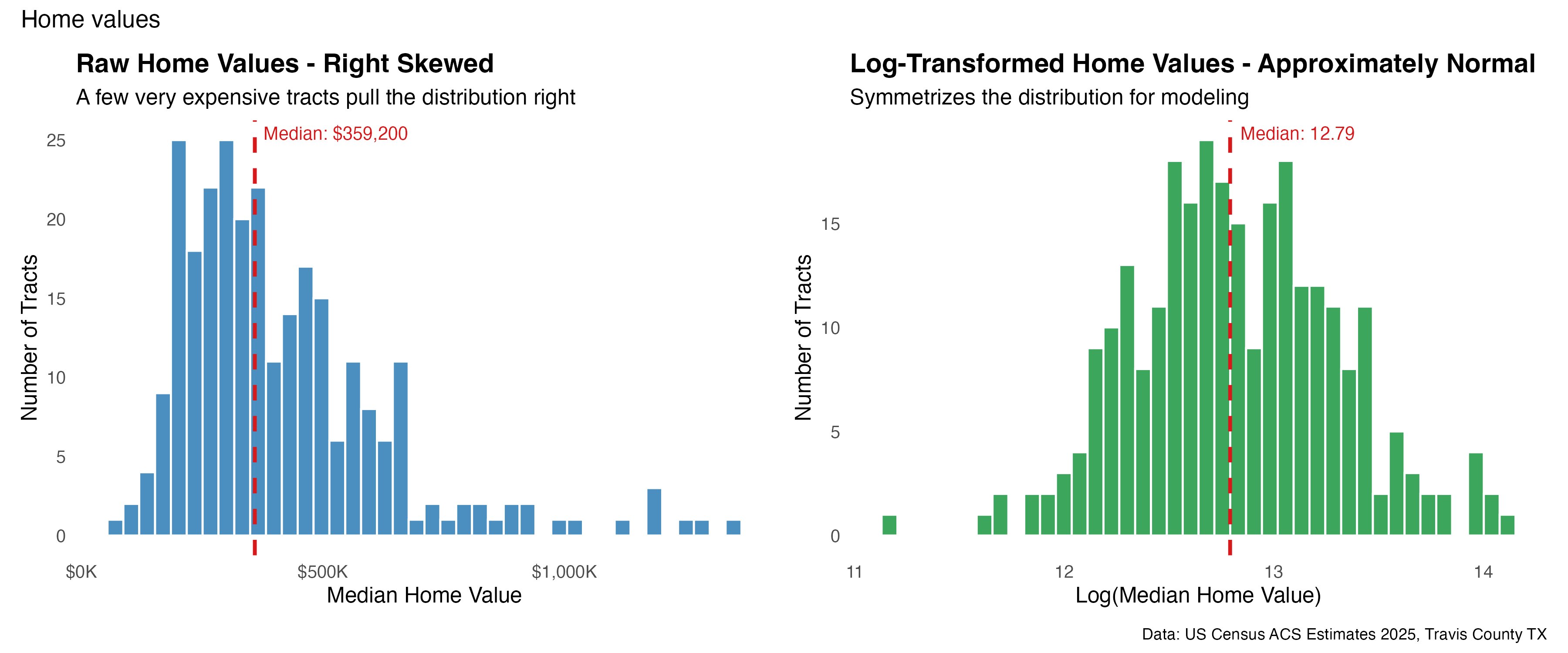
3.1 Why we model the logarithm of price, not price itself
Raw home values are right-skewed: most tracts cluster in an affordable-to-mid range while a handful of luxury neighborhoods stretch far to the right, all the way to $1.35M. Skew like this distorts a regression - the rare expensive tracts pull the model toward themselves and inflate its errors.
The fix is to model the natural logarithm of price. The right-hand panel below shows the payoff: the lopsided distribution becomes a clean, symmetric bell centered at 12.79. As a bonus, working in logs means every coefficient later reads as a percentage effect.
TipIn plain terms
Taking the log is like switching from dollars to percentage changes. It stops a few mansions from dominating the math and lets us say things like “a 1% rise in income lifts prices by 0.4%,” which is far more useful than a raw-dollar slope.
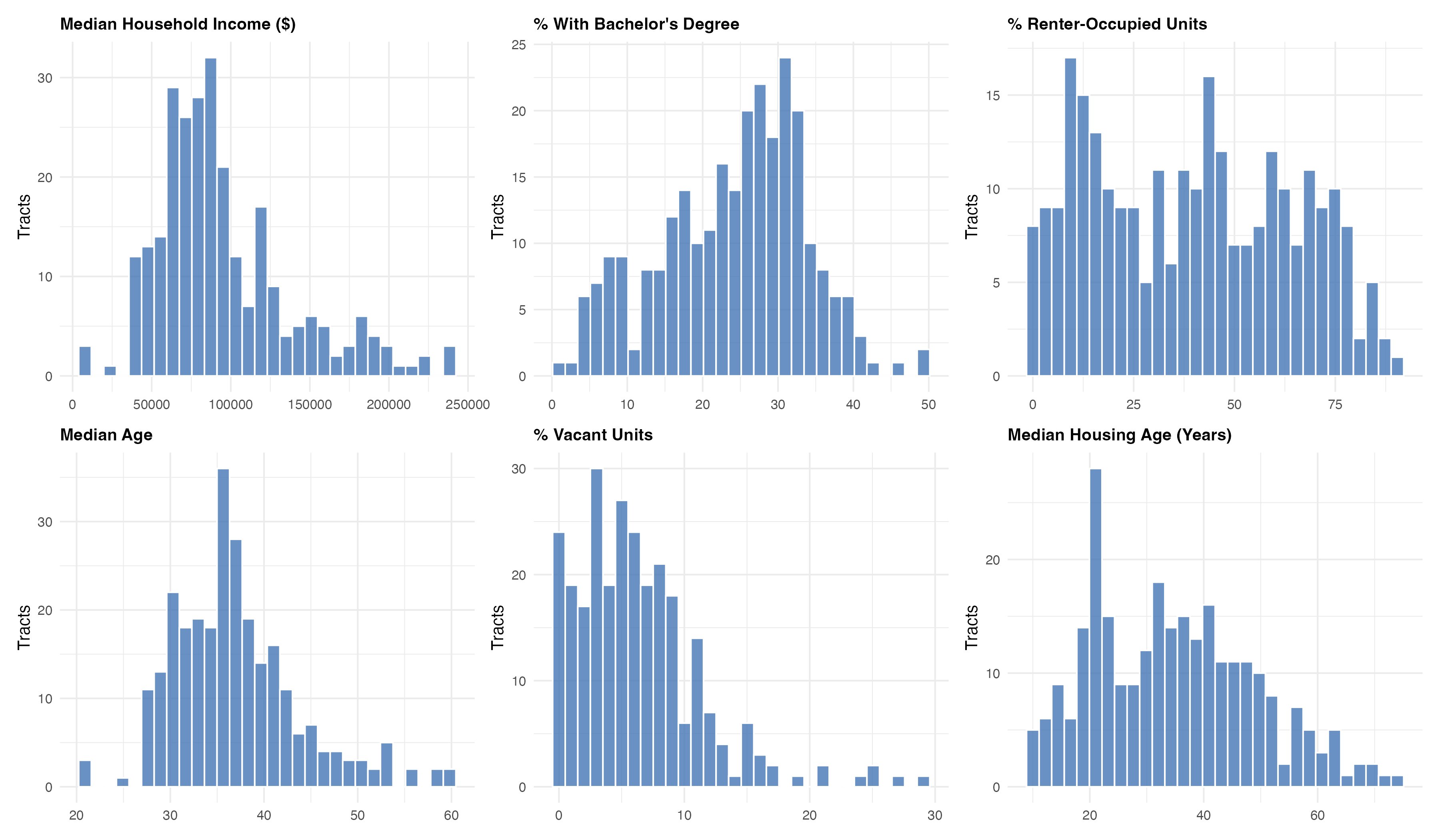
The other predictors show their own shapes - income is right-skewed (a few very wealthy tracts), education is roughly bell-shaped, and rental share is almost bimodal, splitting the county into owner-heavy and renter-heavy neighborhoods.
3.2 Which features actually move prices?
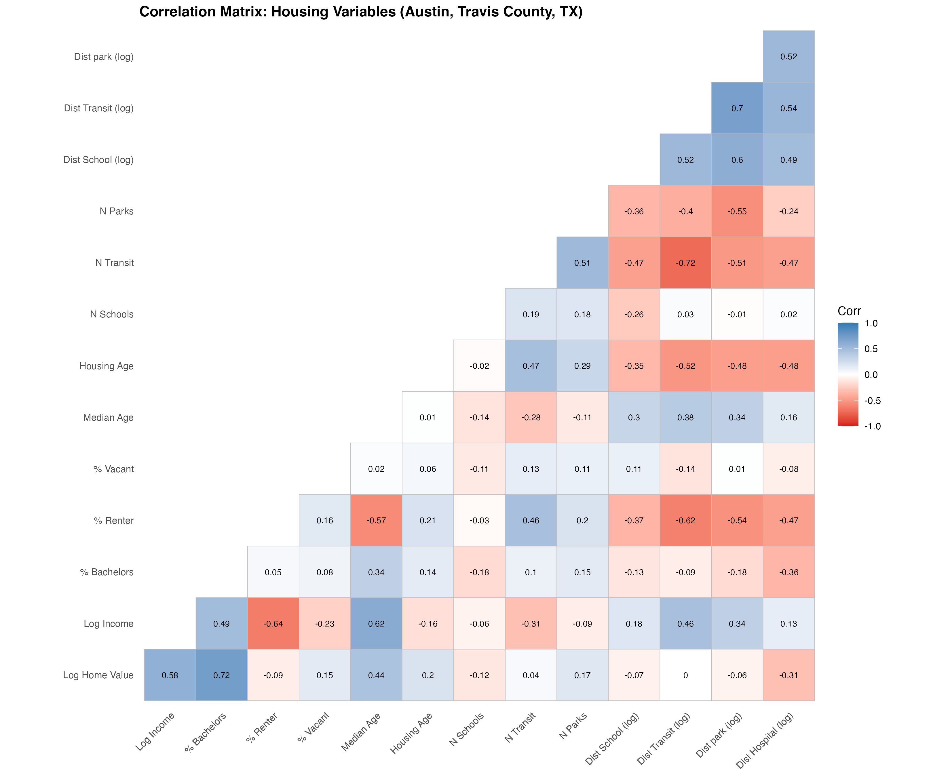
The correlation matrix below measures how strongly each variable tracks home value. Reading the bottom row tells us where the predictive signal lives - and delivers one genuine surprise.
| What correlates with home value? | ||
| r ranges from −1 to +1; further from 0 means a stronger link. | ||
| Variable | Correlation (r) | Interpretation |
|---|---|---|
| % with Bachelor's degree | 0.72 | Strongest signal - education tracks wealth and prices |
| Median income (log) | 0.58 | Strong - richer neighborhoods, pricier homes |
| Median age | 0.44 | Moderate - established, settled areas cost more |
| Distance to hospital | -0.31 | Moderate negative - far from hospitals means the outskirts |
| Median housing age | 0.20 | Weak - older housing isn't necessarily cheaper here |
| Number of parks | 0.17 | Weak positive - green space adds a little value |
| % vacant units | 0.15 | Weak positive - counterintuitive; flagged for the model |
| Number of schools | -0.12 | Weak negative - schools cluster in more affordable areas |
ImportantThe surprise that shaped the whole analysis
Transit access barely correlates with home value at all - distance-to-transit comes in at r = 0.003, transit-stop count at r = 0.04, essentially zero. In a city defined by its traffic, proximity to a bus stop does not move prices at the county scale.
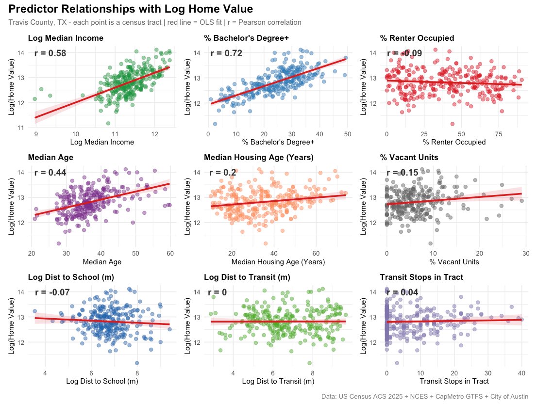
The scatterplots make the strong relationships tangible - education and income climb cleanly with price, while the proximity measures form flat, shapeless clouds.
3.3 The map that makes the case for spatial analysis
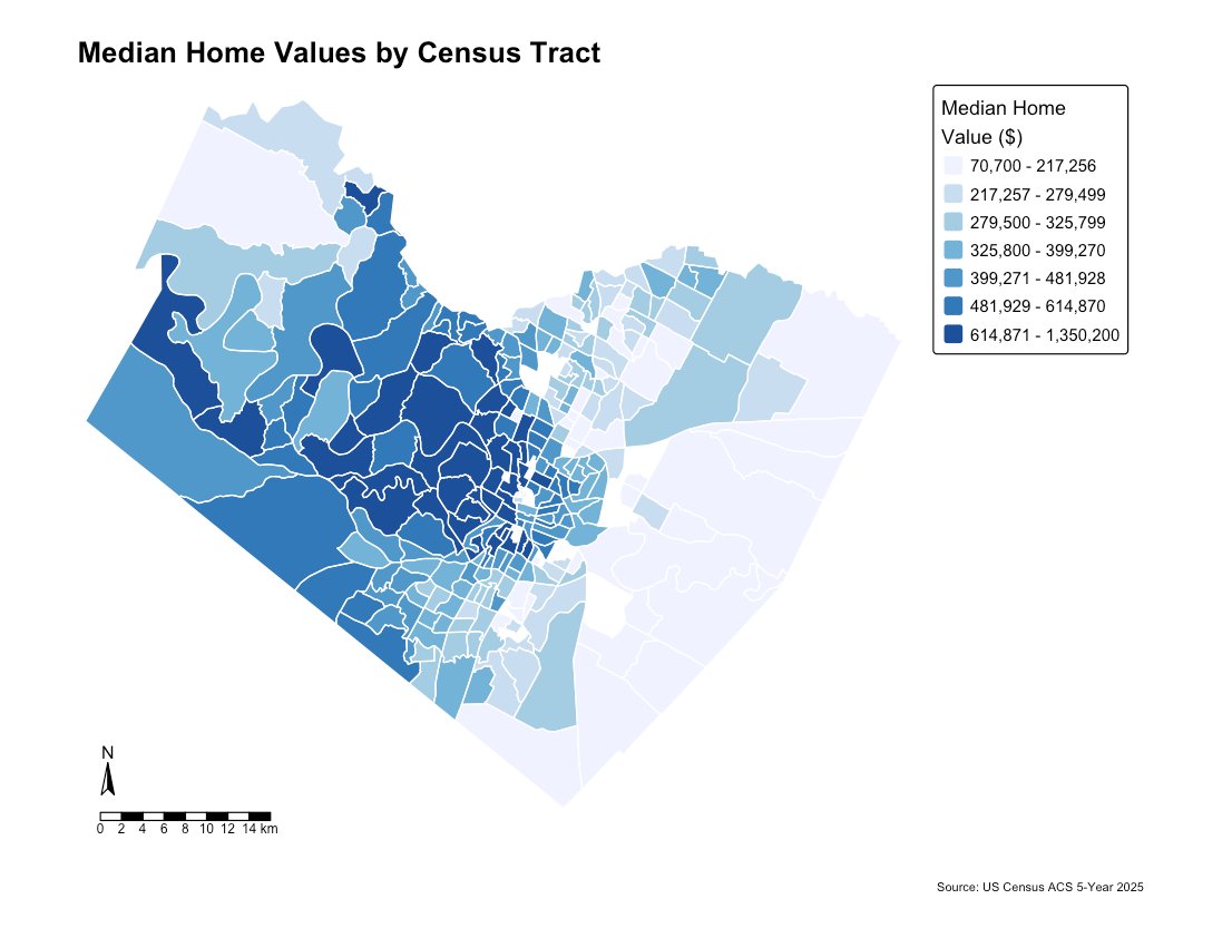
Expensive tracts are not scattered randomly—they are concentrated in central and west Austin, while a contiguous region of affordable tracts is formed to the east. Values are distributed in smooth geographic gradients, resembling a watercolor rather than television static. This smoothness represents spatial autocorrelation, which is visible to the naked eye before a single statistic has been computed.
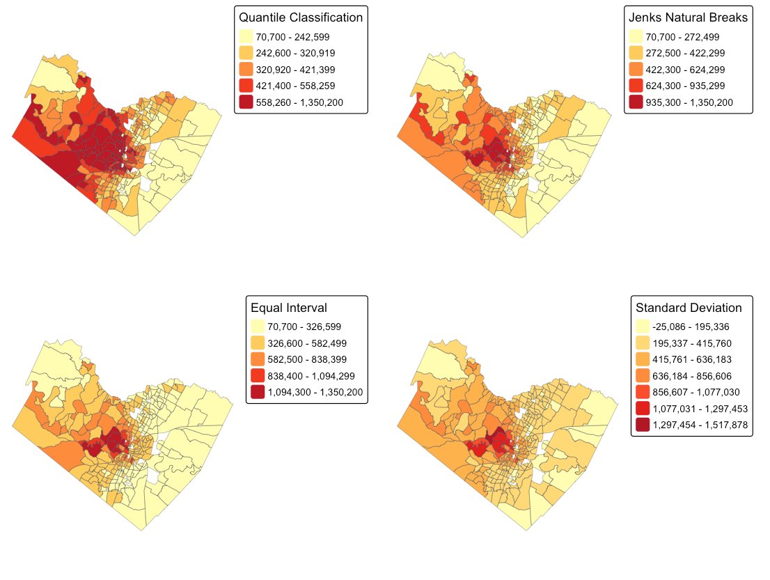
To ensure this pattern is real and not an artifact of how the map was colored, it was re-drawn under four standard classification schemes.
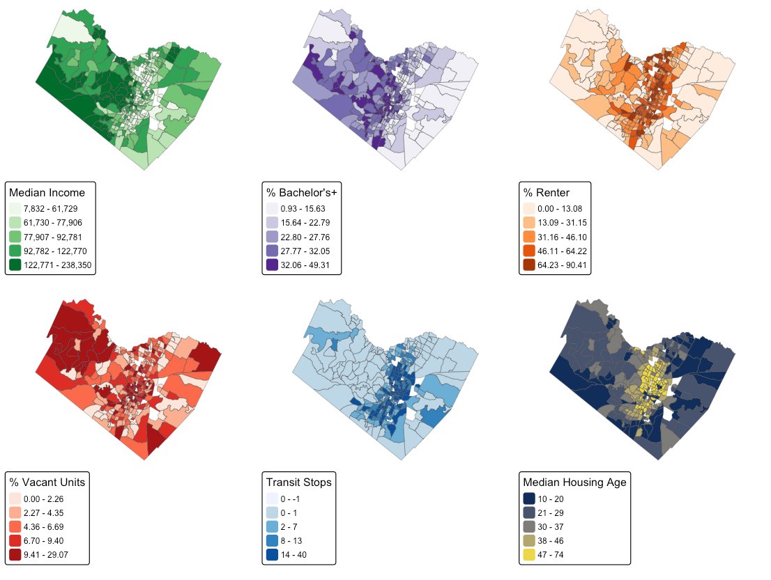
Finally, mapping the predictors side by side shows why the price pattern exists: income, education, and housing age all share the same west-central spine, while the urban core carries its own signature of high rental share and older housing.
4 Measuring the Clustering: Neighbors, Moran’s I, and Local Hotspots
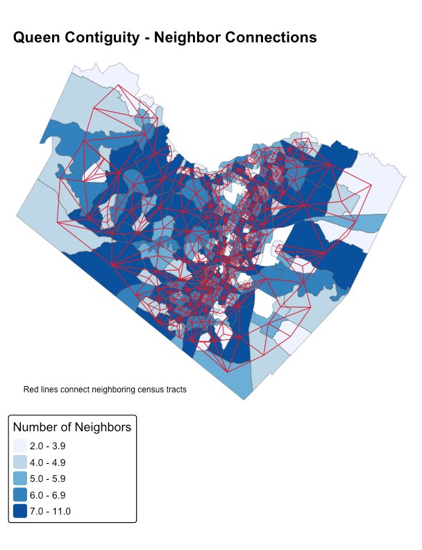
4.1 Defining a neighbor: queen versus rook contiguity
Every spatial statistic rests on which tracts count as neighbors. Rook contiguity counts two tracts as neighbors only if they share a border edge - four neighbors. Queen contiguity also counts tracts that touch at a single corner - up to eight neighbors.

This project uses queen contiguity, because in a real city influence flows in every direction, including diagonally - a luxury development on a corner lot affects the block kitty-corner to it, not just the ones directly adjacent. In code, the neighbor structure and its row-standardized weights are built in two lines:
nb_queen      <- poly2nb(housing, queen = TRUE)        # find neighbors
weights_queen <- nb2listw(nb_queen, style = "W")       # row-standardize
The resulting network is fully connected - 269 tracts joined by 1,552 neighbor links, averaging 5.77 neighbors each (ranging from 2 to 11), with no isolated tracts to drop from the analysis.
4.2 The headline measure of clustering: Global Moran’s I
With neighbors defined, Global Moran’s I asks a single question: do tracts resemble their neighbors more than they resemble random tracts elsewhere? It runs from −1 (perfect checkerboard) through 0 (no pattern) to +1 (strong clustering). It was computed, then stress-tested with a Monte Carlo simulation—home values were randomly reshuffled across the map 999 times to determine how often pure chance could replicate this much clustering.
moran.mc(housing$log_home_value, listw = weights_queen, nsim = 999)| Global Moran’s I - tested against 999 random shuffles | |
| Measure | Result |
|---|---|
| Observed Moran's I | 0.6966 |
| Average I under random shuffling | −0.0030 |
| How our result ranked | 1st out of 1,000 |
| Probability it's due to chance | 0.001 (the lowest possible) |
ImportantWhat this means
Austin’s home values score a Moran’s I of 0.70 - and across 999 random reshuffles, not one produced clustering anywhere near this strong. To put 0.70 in context: in social-science data, anything above 0.3 is considered strong clustering. 0.70 is exceptional. Austin’s housing geography is about as spatially structured as real-world data ever gets, and the probability this arose by chance is effectively zero.
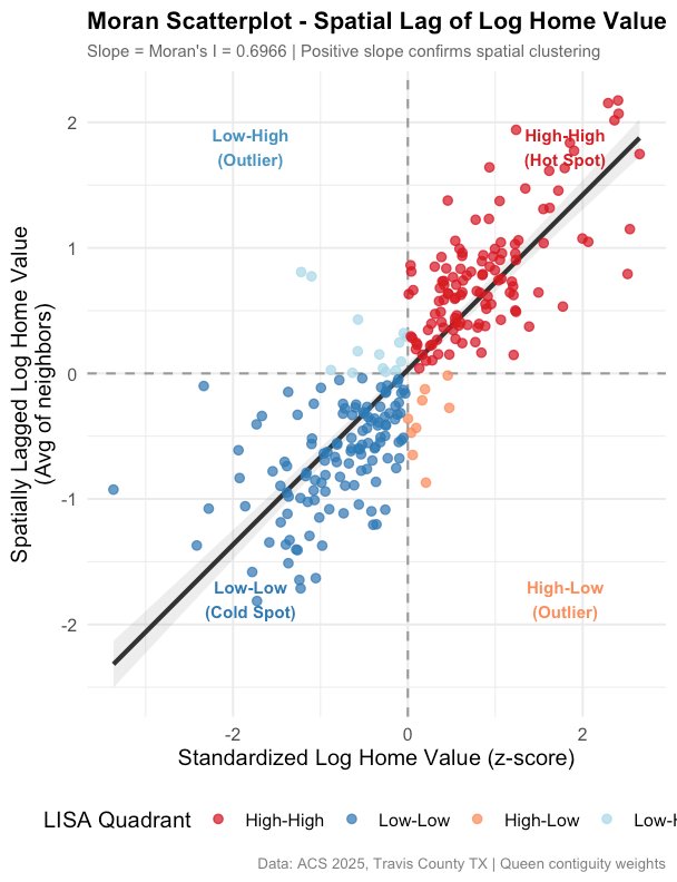
The Moran scatterplot transforms that single number into a visual representation. Each tract’s own value is plotted on the horizontal axis; the average value of its neighbors is plotted on the vertical axis. The slope of the resulting cloud represents Moran’s I. The conceptual diagram below explains the meaning of each of the four quadrants before the real data is examined.

NoteReading the four quadrants
A tract lands in the top-right (High–High) if it is expensive and surrounded by expensive neighbors - a hot spot. The bottom-left (Low–Low) is the opposite - an affordable tract among affordable neighbors, a cold spot. The two off-diagonal quadrants are spatial outliers: a lone expensive tract in a poor area (High–Low) or a lone affordable tract in a rich area (Low–High). Strong positive clustering means most tracts fall on the High–High / Low–Low diagonal.
The real Moran scatterplot for Austin confirms it: a tight, upward-sloping cloud dominated by the High–High and Low–Low quadrants.
4.3 Pinpointing the clusters: Local Moran’s I (LISA)
Global Moran’s I proves clustering exists somewhere. LISA (Local Indicators of Spatial Association) proves where, by computing a miniature Moran’s test for every individual tract and flagging the statistically significant clusters.
| LISA cluster classification (significant at p < 0.05) | |||
| Cluster type | Tracts | Share | Where |
|---|---|---|---|
| High–High (hot spot) | 45 | 16.7% | Central & west Austin |
| Low–Low (cold spot) | 40 | 14.9% | Eastern county |
| High–Low (outlier) | 1 | 0.4% | A single tract |
| Not significant | 183 | 68.0% | No significant local pattern |
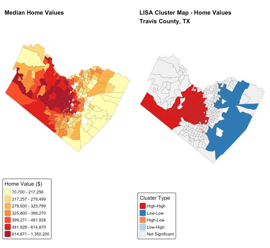
ImportantThe geography of inequality, made measurable
Austin divides into two large, contiguous economic zones - a 45-tract high-value cluster in the central and western county, and a 40-tract low-value cluster across the east. This is the statistical signature of Austin’s well-documented east–west divide, a separation rooted in the city’s 1928 master plan and still clearly measurable in home values nearly a century later. Tellingly, there is exactly one outlier tract and no affordable islands inside the wealthy core - the segregation of value is almost complete.
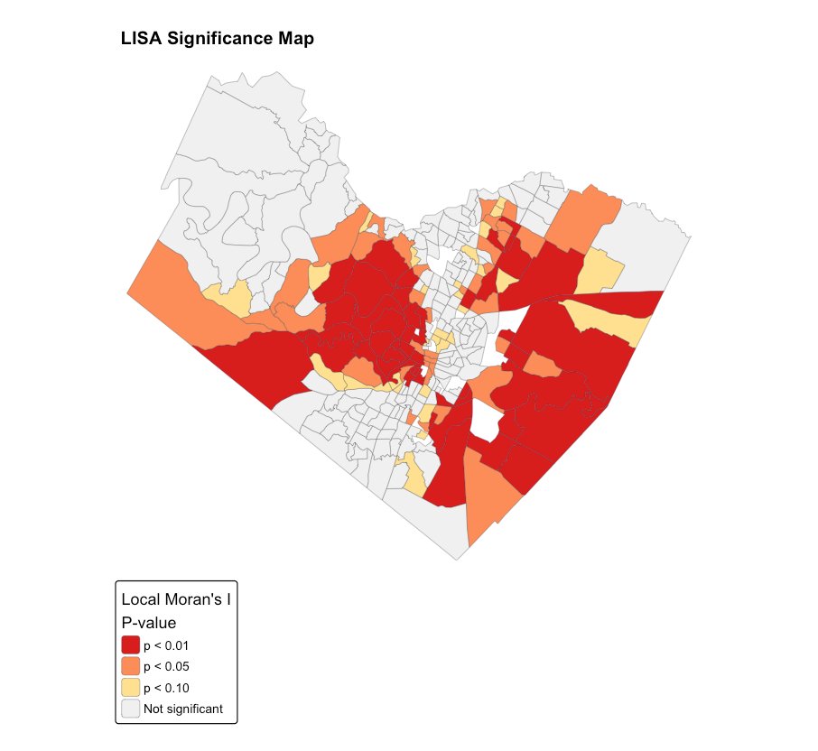
The significance map confirms these clusters are statistically solid: the deepest-red tracts are significant at p < 0.01.
5 Why a Standard Regression Model Fails Here
5.1 The baseline model and what its coefficients say
We model log home value as a function of income, education, tenure, housing characteristics, and amenity proximity. To make the results readable, the table below groups the coefficients into the three forces that drive a home’s price. Each coefficient is a ceteris paribus effect - its influence holding all the other variables constant.
| OLS coefficients, grouped by what they represent | ||
| Each effect is 'all else equal.' R² = 0.676 · Adjusted R² = 0.664 · AIC = 99.3 | ||
| Variable | Coefficient | Significant1 |
|---|---|---|
| Economic capacity | ||
| Log median income | 0.5908 | Yes *** |
| Neighborhood quality | ||
| % with Bachelor's degree | 0.0177 | Yes *** |
| % vacant units | 0.0204 | Yes *** |
| % renter-occupied | 0.0049 | Yes *** |
| Housing age | 0.0063 | Yes *** |
| Median age | 0.0072 | Borderline |
| Accessibility (amenities) | ||
| Distance to school | -0.0288 | No |
| Distance to transit | 0.0036 | No |
| Distance to park | -0.0019 | No |
| Transit-stop count | -0.0020 | No |
| 1 *** = statistically significant at p < 0.001. | ||
- Economic capacity is the dominant force. The income coefficient of 0.59 means that, all else equal, a 1% rise in a neighborhood’s median income is associated with roughly a 0.59% rise in home values.
- Neighborhood quality matters and is highly significant: more college graduates, older established housing, and - counter intuitively - higher vacancy all align with higher values (vacancy here is likely flagging high-turnover, in-demand central neighborhoods rather than distress).
- Accessibility is the dog that didn’t bark. Every amenity-distance variable is statistically insignificant at the county scale. This echoes the correlation surprise from earlier, and the spatial models will explain why.
5.2 Reading the diagnostic plots - what each one is testing
A regression is only trustworthy if its assumptions hold. The four diagnostic panels below each test a different assumption. Understanding what each is for is the difference between trusting a model and being fooled by one.
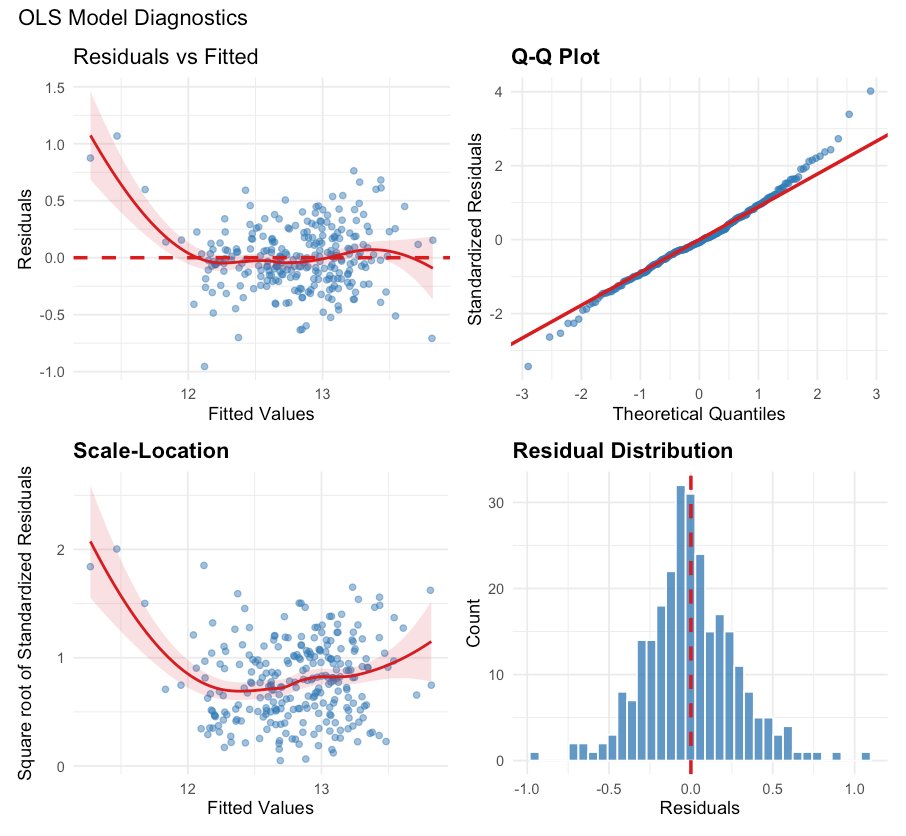
NoteWhat each panel is checking
① Residuals vs Fitted (top-left) - tests for a straight-line relationship. If the model captured the structure, this should be a flat, patternless band around zero. Instead the red trend line curves at the low-price end, a sign the model misses something for the cheapest tracts - it slightly over-predicts them.
② Normal Q–Q plot (top-right) - tests whether errors are normally distributed. If the residuals are normal, the points hug the diagonal. They mostly do, but the upper tail lifts above the line: a handful of tracts are far more expensive than the model expects - the luxury outliers.
③ Scale–Location (bottom-left) - tests for constant error variance (homoscedasticity). A trustworthy model spreads its errors evenly across all price levels, giving a flat line. Here the line dips then rises, meaning the model is more uncertain at the extremes than in the middle - its confidence intervals can’t be taken at face value.
④ Residual histogram (bottom-right) - the overall error distribution. Centered near zero and roughly bell-shaped, which is reassuring, but with the slight heavy tails the other panels already flagged.
These classical diagnostics indicate a model that is strained but not obviously broken. The decisive failure only becomes apparent when the residuals are examined on a map.
5.3 The smoking gun: errors that cluster in space
For geographic data, the most important question is one the classical plots never ask: are the model’s mistakes spatially clustered? If the model over-predicts in whole regions and under-predicts in others, its errors aren’t independent - and the entire statistical foundation of OLS collapses. The interactive map below shows the OLS residuals; pan and hover to explore where the model misses.
The errors are clearly not random noise - they form coherent geographic patches. This was formally confirmed by running Moran’s I on the residuals themselves:
lm.morantest(ols_model, listw = weights_queen)| Testing the OLS residuals for spatial clustering | |
| Test | Result |
|---|---|
| Moran's I of the OLS residuals | 0.3218 |
| Probability this is due to chance | less than 1 in 10 billion |
| Verdict | The errors are strongly clustered - OLS is statistically invalid here |
ImportantThis is the turning point of the project
The OLS residuals carry a Moran’s I of 0.32 with a probability below one-in-ten-billion of arising by chance. In plain terms: when the model is wrong, it is wrong in whole neighborhoods at once. That violates the core assumption that observations are independent. The consequences are real - the coefficients are biased, the standard errors are too small, and the model is quietly overconfident. A respectable-looking R² of 0.68 was hiding a fatal flaw. We need a model that builds geography into its very structure.
6 Choosing the Right Spatial Model
If geography must be built into the model, the question becomes how. There are two principled ways to do it, and the data itself can tell us which one fits. This section lays out the mathematics in plain terms, lets a formal test pick the model, and compares the results head to head.
6.1 The three models, in math and in words
A standard regression assumes each tract stands alone:
y = X\beta + \varepsilon
Here y is log home value, X holds the predictors, \beta are the coefficients (the “levers”), and \varepsilon is the random error. There is no geography anywhere in that equation - which is exactly why it failed.
The Spatial Lag Model (SLM) adds one term that encodes the neighborhood:
y = \rho W y + X\beta + \varepsilon
The new piece, \rho W y, is the average home value of each tract’s neighbors (Wy) multiplied by a spillover strength \rho (rho). In words: a tract’s price is partly set by the prices around it. This is the right model when neighboring values genuinely influence one another - exactly how housing markets behave, as buyers price a home by looking at recent sales next door.
The Spatial Error Model (SEM) instead places the geography in the error term:
y = X\beta + u, \qquad u = \lambda W u + \varepsilon
Here \lambda (lambda) captures spatial correlation among unmeasured factors - a shared “neighborhood feel,” school reputation, or local amenities the data doesn’t contain. This is the right model when the clustering comes from missing variables rather than genuine spillover.
TipIn plain terms
SLM says neighbors’ prices push on each other directly. SEM says neighbors share hidden characteristics the model can’t see. Both fix the clustered-error problem; they just tell different stories about why the clustering exists.
6.2 Letting the data choose: the Lagrange Multiplier tests
Rather than guess, we run Lagrange Multiplier (LM) tests - formal diagnostics that examine the OLS residuals and score how much each type of spatial model is needed. The procedure (the Anselin decision tree) compares the plain and “robust” versions of each test to break ties.
lm.LMtests(ols_model, listw = weights_queen,
test = c("LMlag","LMerr","RLMlag","RLMerr"))| Lagrange Multiplier tests for spatial structure | ||
| All four fire strongly; the robust comparison pointed to the Spatial Lag Model. | ||
| LM test | Test statistic | Significant? |
|---|---|---|
| Spatial-lag dependence | ≈ 129 | Yes *** |
| Spatial-error dependence | ≈ 129 | Yes *** |
| Robust lag | ≈ 129 | Yes *** |
| Robust error | ≈ 129 | Yes *** |
Every test fired decisively (all p < 0.001), confirming that some spatial model is essential. The robust comparison favored the Spatial Lag Model, so it is treated as the lead specification—but both are fitted and compared honestly below.
6.3 The three models, side by side
The table below is the single most important comparison in the project. Each row is a model; each column answers a specific question. Lower AIC means a better fit. Pseudo-R² is the share of variation explained. Residual Moran’s I should sit near zero if the model has successfully absorbed the spatial clustering.
| OLS vs. Spatial Lag vs. Spatial Error | |||||
| The spatial models don't just fit better - they repair the flaw that made OLS invalid. | |||||
| Model | Fit (AIC, lower is better) | Variation explained | Neighborhood strength | Leftover clustering (Moran's I) | Did it fix the clustering? |
|---|---|---|---|---|---|
| OLS - standard regression | 99.30 | 67.6% | none | 0.32 | No - still clustered |
| Spatial Lag (SLM) | −13.20 | 80.3% | rho = 0.57 | −0.03 | Yes - errors now random |
| Spatial Error (SEM) | 0.90 | 81.0% | lambda = 0.78 | −0.06 | Yes - errors now random |
ImportantWhat the comparison shows
Both spatial models completely repaired the flaw that doomed OLS. The leftover clustering in the residuals collapsed from a damning 0.32 to a harmless −0.03 (SLM) and −0.05 (SEM) - statistically indistinguishable from random noise, which is exactly the goal. Fit improved dramatically too: the Spatial Lag Model’s AIC fell from 99.3 to −13.2 (any drop beyond 10 points is considered decisive), and the variation explained rose from 68% to 80%. The neighborhood-strength term rho = 0.57 is large and highly significant, confirming that a tract’s value is powerfully shaped by its neighbors’.
7 How a Change in Income Ripples Through the Market
Here is where spatial modeling earns its keep. In an ordinary regression, raising a variable in one tract affects only that tract. In a spatial model, the effect spreads - and quantifying that spread reveals how a neighborhood’s fortunes are tied to its neighbors’.
7.1 Why a coefficient is no longer the whole story
In OLS, the income coefficient of 0.59 is the complete answer: raise income, raise that tract’s value, done. But the Spatial Lag Model says a tract’s value depends on its neighbors’ values - so the story compounds. When income rises in one tract, its own value rises (the direct effect); that higher value then nudges up its neighbors’ values through the \rho W y term; those higher neighbor values nudge back, and so on. The full chain is captured by what’s called the spatial multiplier:
\text{total effect} = (I - \rho W)^{-1}\,\beta
That formula sounds abstract, but it cashes out into three intuitive quantities for each variable:
- the direct effect - the impact on a tract’s own value,
- the indirect (spillover) effect - the combined impact on all its neighbors,
- the total effect - the two added together.
impacts(slm_model, listw = weights_queen, R = 1000) # simulate the spillovers| Direct, indirect, and total effects on home value | ||||
| How a 1-unit rise in each variable ripples through the spatial system (significant effects shown). | ||||
| Variable | Direct (own tract) | Indirect (neighbors) | Total effect | Share that spills over |
|---|---|---|---|---|
| Income | 40.6% | 46.5% | 87.0% | 53% |
| % Vacant units | 1.03% | 1.18% | 2.22% | 53% |
| % Bachelor's degree | 0.99% | 1.13% | 2.12% | 53% |
| % Renter | 0.25% | 0.28% | 0.53% | 53% |
ImportantMore than half of income’s effect lands next door
Income’s total effect on home value is a remarkable 87% - but only 40.6% of that acts on a tract’s own value. The other 46.5% spills over onto neighboring tracts. Put differently: 53% of the value created by rising income flows to the neighbors, not the source. For a buyer, this means a property’s worth is driven as much by who is moving in next door as by its own block. For a city planner, it is a hard number justifying place-based investment: money put into one neighborhood radiates value across the ones around it.
7.2 The same change, seen through four models
Because each model treats geography differently, each gives a different - and progressively richer - answer to the simple question, “what happens to home values if a neighborhood’s income rises by 1%?”
| One question, four answers: the effect of rising income | ||
| Model | What a 1% rise in income does | Spillover? |
|---|---|---|
| OLS | A flat 0.59% rise in that tract - same everywhere, no spillover. | No |
| Spatial Error (SEM) | About 0.40% in that tract - same everywhere, but estimated more efficiently. | No |
| Spatial Lag (SLM) | 0.37% directly plus 0.47% spilling to neighbors = 0.87% total across the system. | Yes - 53% |
| Geographically Weighted (GWR) | Anywhere from 0.07% to 1.27% depending on the neighborhood - the effect is local. | Varies by place |
The progression tells its own story. OLS sees one rigid number. SEM refines it. SLM reveals the spillover. And GWR - the subject of the next section - discovers that the number isn’t fixed at all.
8 Where the Rules Change: Geographically Weighted Regression
Every model so far assumes one rulebook for the entire county - that income, education, and the rest matter exactly as much in wealthy west Austin as in the eastern flatlands. Geographically Weighted Regression (GWR) abandons that assumption and asks a more honest question: what if the rules themselves change from place to place?
8.1 The idea behind GWR
Instead of fitting one regression for all 269 tracts, GWR fits a separate mini-regression centered on every single tract, each one giving more weight to nearby tracts and less to distant ones. The “how nearby counts” is set by two choices:
- a bisquare kernel, a smooth weighting curve that fades a tract’s influence to zero past a certain distance, and
- an adaptive bandwidth of 69 neighbors, chosen automatically by cross-validation - meaning each local regression learns from its 69 closest tracts.
bw  <- bw.gwr(formula, data = housing_sp, adaptive = TRUE, kernel = "bisquare")
gwr <- gwr.basic(formula, data = housing_sp, bw = bw, adaptive = TRUE)
The result is not one coefficient per variable but a coefficient surface - a whole map of how each effect varies across the city.
TipIn plain terms
A global model is like quoting one nationwide price for an extra bedroom - useful on average, useless on any actual street. GWR is like having a local appraiser stationed in every neighborhood, each quoting the price that truly applies there. Real estate is local; GWR finally lets the model be local too.
8.2 How much better does it fit?
0.90Variation explained (up from 0.68)
0.88Median local fit
0.99Best local fit
269 / 269Tracts fitting above 0.75
GWR lifts the explained variation from the OLS figure of 68% to a remarkable 90%, and every tract is explained well (local fit above 0.75 everywhere). The model succeeds everywhere precisely because it uses different coefficients in different places.
8.3 What the coefficient maps reveal
The maps below show where each force is strongest. Only the statistically significant tracts are colored; grey areas are where that variable doesn’t significantly move prices.
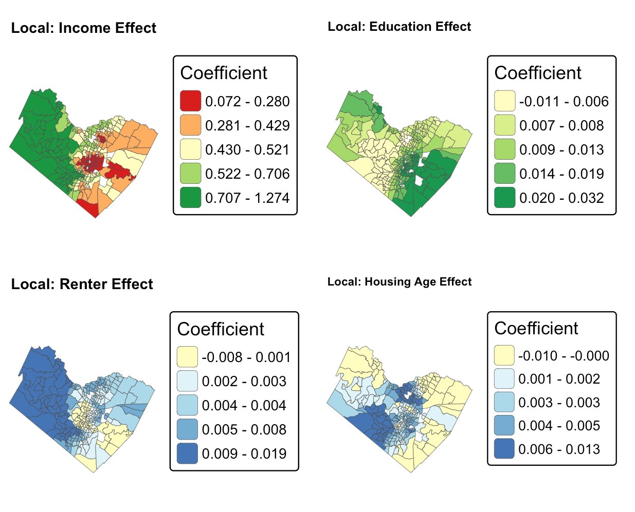
The income map carries a subtle, sophisticated insight. Income’s effect is weakest in the wealthy central core - where nearly everyone is high-income, so income no longer distinguishes one tract from another - and strongest at the transitional edges, where income differences still sharply sort neighborhoods. That is the spatial signature of a city in the middle of economic change.
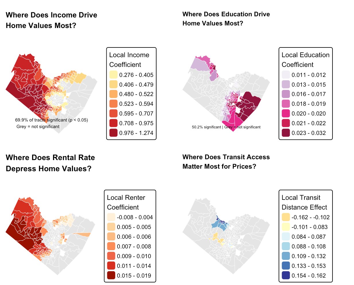
ImportantGWR solves the transit mystery
Recall that transit access showed essentially zero correlation with home value across the county. GWR reveals the truth: transit proximity has a strong effect, but only inside a handful of central tracts, where its local coefficient swings from −0.16 to +0.16. Averaged across all 269 tracts, that intense but localized effect cancels out to nothing. The global model wasn’t wrong so much as blind - it could only see the average, and the average hid the real, geographically concentrated story.
9 Reconciling the Models: Why a 90% R² Doesn’t Crown GWR
GWR explains 90% of the variation in home values and the Spatial Lag Model explains only 80% - so why is SLM, not GWR, named the final predictive model? The answer is one of the most important judgment calls in the whole project, and resolving it cleanly is what separates a model that looks best from the one that actually is best for the job.
| The apparent contradiction | ||
| On raw fit, GWR seems to win. Three things complicate that conclusion. | ||
| Model | Variation explained (raw R²) | Reported information criterion |
|---|---|---|
| Spatial Lag (SLM) | 80.3% | AIC = −13.2 |
| GWR | 89.7% | AICc = 58.7 / AIC = −140.3 |
Three considerations dissolve the contradiction and once they are accounted for, SLM is clearly the right choice for prediction.
9.1 First: AIC and AICc, and why they can’t be compared across model families
Both AIC and AICc are scores for ranking models, and for both, lower is better. They work by balancing the two things a good model must trade off - how well it fits, and how complex it is.
The Akaike Information Criterion (AIC):
\text{AIC} = -2\log(L) + 2k
The first term rewards fit (it shrinks as the model matches the data better); the second term, 2k for k parameters, is a penalty for complexity. The logic is that any model can fit better simply by adding parameters, so AIC charges two points per parameter - a parameter only improves the score if it earns its keep. This is what guards against being fooled by an over-fit model.
The small-sample correction (AICc):
\text{AICc} = \text{AIC} + \frac{2k(k+1)}{n-k-1}
Plain AIC under-penalizes complexity when there are few data points per parameter. AICc adds a correction that grows as k approaches the sample size n and fades to zero for large samples. The standard guidance is to prefer AICc whenever n/k is below about 40.
This is precisely GWR’s situation. Its diagnostics report an effective number of parameters of 118.7 against just 269 data points - barely two observations per parameter, deep in the small-sample regime AICc was built for. That is why GWmodel reports AICc, and why bw.gwr() minimizes AICc when choosing the bandwidth.
ImportantWhy the AIC comparison is invalid here
GWR reports two different information criteria - AICc = 58.7 and AIC = −140.3 - because they come from different formulas in Fotheringham’s GWR framework. Compare SLM’s −13.2 to the first and GWR looks worse; compare it to the second and GWR looks better. The fact that the verdict flips depending on which GWR number you grab is the tell: GWR’s criteria are built on an effective-degrees-of-freedom likelihood, while OLS, SLM, and SEM use a single global Gaussian likelihood. They are not on the same scale. AIC is the right tool for comparing the global models to each other - but ranking SLM against GWR by AIC is apples to oranges, and cannot be used to declare a winner.
9.2 Second: GWR’s 90% is inflated by its own flexibility
A model with roughly 119 effective parameters will almost always post a higher in-sample R² than one with 12 - that is flexibility, not superior insight, and flexibility shades into overfitting. The honest comparison uses the penalized fit measures that charge each model for its complexity:
| Raw versus penalized fit | |||
| Once GWR is charged for its complexity, the gap nearly disappears. | |||
| Model | Effective parameters | Raw fit | Penalized fit |
|---|---|---|---|
| Spatial Lag (SLM) | ~12 | 0.803 (pseudo-R²) | 0.803 |
| GWR | ~119 | 0.897 (R²) | 0.816 (adjusted R²) |
GWR’s adjusted R² of 0.816 sits almost exactly on SLM’s pseudo-R² of 0.803. The eye-catching 0.897 was the headline; 0.816 is the figure that accounts for the ~119 parameters GWR spent to get there. Statistically, the two models explain the data about equally well - GWR simply paid far more for the privilege.
9.3 Third - and decisively: the final model is judged on out-of-sample prediction
“Final model for prediction” has a precise meaning: how well does it forecast values it has never seen? That is measured on held-out data, not on the data the model was fit to. In-sample R² (where GWR shines) measures how well a model memorizes its training data; out-of-sample error measures how well it generalizes. For a prediction task, only the second one counts - and there, SLM won cleanly, with the lowest error of any model (MAPE 19.6%, RMSE ≈ $124,812).
GWR is also genuinely awkward as a predictor by design. Its entire apparatus is the set of local coefficients estimated at the 269 observed tracts; forecasting a brand-new location requires interpolating or recalibrating those surfaces, the prediction variance is large, and the local coefficients can be unstable. GWR’s local income effect swings from 0.07 to 1.27 and education even turns negative in places. Some of that is real heterogeneity; some is noise from slicing 269 points into 269 tiny regressions. SLM, by contrast, has one clean generative equation, valid standard errors, and a direct prediction path.
9.4 The resolution: the two models have different jobs
| One project, two final models - for two different purposes | ||
| Model | Role | Why it holds that role |
|---|---|---|
| Spatial Lag (SLM) | Final predictive model | Parsimonious, interpretable, statistically valid (residual Moran’s I = −0.027, p = 0.74), best out-of-sample accuracy, and it yields the direct/indirect/total spillover decomposition. |
| GWR | Final explanatory model | Reveals where the rules of the market change - income matters most at the transitional edges and least in the saturated core, and it exposes the localized transit effect the global models were blind to. |
10 How Accurately Can We Predict Home Values?
10.1 Predicted versus actual, tract by tract
The plot below pairs every tract’s predicted value against its true value. Points hugging the diagonal line are accurate predictions; the tighter the cloud, the better the model. Hover any point to read off that tract’s numbers.
10.2 The prediction map
The same predictions, placed back on the map. Comparing this surface against the actual-value map.
10.3 The accuracy scorecard
To compare models fairly, we convert their predictions back into dollars and measure the typical error. RMSE and MAE are average dollar misses (lower is better); MAPE is the average miss as a percentage of the home’s value - the most intuitive single number.
| Prediction accuracy, in real dollars | ||||
| Model | Typical $ error (RMSE) | Average $ error (MAE) | Average % error (MAPE) | Verdict |
|---|---|---|---|---|
| OLS | $136,194 | $91,467 | 22.8% | Baseline |
| Spatial Lag (SLM) | $124,812 | $80,174 | 19.6% | Most accurate |
| Spatial Error (SEM) | $163,725 | $109,348 | 26.7% | Best fit, weaker prediction |
ImportantThe Spatial Lag Model wins where it counts
The Spatial Lag Model is the most accurate predictor, cutting the average error from OLS’s 22.8% to 19.6% - a 14% improvement - and trimming the typical dollar miss by over $11,000 per tract. Interestingly, the Spatial Error Model had a marginally better statistical fit yet predicted worse in dollars. For the practical task of valuing a home, SLM is the clear choice.
11 What This Means for Buyers, Planners, and Lenders
| From statistics to decisions | |
| For a… | The takeaway |
|---|---|
| Home buyer | Because 53% of income's effect spills to neighbors, the smart buy is on the rising edge of an appreciating cluster - where GWR shows income still has room to lift prices - not its already-saturated core. |
| City planner / policymaker | The east–west divide is a measurable, century-old inequality. The 53% spillover means investment in one neighborhood radiates value outward, strengthening the case for place-based programs. |
| Mortgage lender | A spatial model cuts valuation error by 14%. On a loan book, that is a direct, compounding reduction in risk on every automated property valuation. |
| Data scientist | Always test residuals for spatial clustering on geographic data. Here, a healthy-looking R² of 0.68 concealed a fatal flaw that a single diagnostic exposed. |
12 Limitations and Where This Goes Next
- These are neighborhoods, not houses. Census tracts are aggregates, so the findings describe areas, not individual homes.
- It is a snapshot, not a trend. The data captures a single ACS period, so it cannot say whether the east–west divide is widening or narrowing. A spatio-temporal model across multiple years is the natural next step.
- Some price drivers are missing. There is no square footage, bedroom count, or build quality here - the staples of a true home appraisal. Part of why the spatial term works so hard is that it absorbs the geographic shadow of those missing variables.
- Transit defies a single summary. Because it matters locally but not globally, no one number captures it; GWR handles this, but a production model would add explicit spatial-interaction terms.
The clearest next steps are an interactive dashboard letting users toggle between models live, a multi-year extension to model change in affordability, and the addition of parcel-level housing characteristics to build a true automated valuation model.
13 Conclusion
This project set out from a problem felt across the country - that a home is slipping out of reach and narrowed it to a precise, answerable question: what makes a home in one Austin neighborhood worth so much more than the same home in another?
The answer is that geography is not a footnote to the price; it is a primary author of it. Home values cluster with a Moran’s I of 0.70, splitting Travis County into two contiguous economic zones along a line drawn a century ago. A conventional regression, for all its respectable 68% fit, proved statistically invalid - its errors clustered in space, betraying that it had missed the most important feature of the data. Rebuilding the model to embrace geography - through a Spatial Lag Model, and then through Geographically Weighted Regression - repaired that flaw, lifted the explained variation to 90%, and cut real prediction error by 14%.
The deeper lesson is that the spatial models did not merely predict better; they explained more. They revealed that over half of income’s effect on home value spills across property lines, that transit matters intensely but only in pockets the global view rendered invisible, and that the very rules of the market shift as you move across the city.
Methods: R · sf · spdep · spatialreg · GWmodel · gstat · tmap · ggplot2 · leaflet · Quarto
Data: US Census ACS 5-Year · NCES EDGE · CapMetro GTFS · City of Austin Open Data · DataLumos
Analysis and report by Sailaxman Kotha · Full code available on Github
Data: US Census ACS 5-Year · NCES EDGE · CapMetro GTFS · City of Austin Open Data · DataLumos
Analysis and report by Sailaxman Kotha · Full code available on Github